This article covers a small but important part of game physics that concerns simulating rigid bodies in time, without taking into account any constraints or collisions. Since linear motion of rigid bodies is pretty simple, we are only concerned about their rotational behavior. The rotational motion is actually very rich and interesting, and its non-linear behaviors are often disregarded by physics engines in favor of a simple implementation. The lack of correct rotational motion is hard to notice but leads to an annoying phenomenon: unrealistically spinning poles.

Truck tumbling around its intermediate principal axis of inertia
Long poles don’t have the correct mass distribution to have a stable angular velocity vector, and this is the crux of the problem: without the presence of forces, angular velocities are non-constant unlike linear velocities. The difference comes from the fact that the mass is invariant under translation but the world space moment of inertia is not invariant under rotation.

Dancing Pole: Weird (Euler integrator)

Ok (Implicit Runge Kutta Integrator). Both simulations start with the same initial angular velocity.
Unfortunately the rotational equations of motion are highly non-linear and difficult to integrate directly; it is much more approachable to use a numerical method. This article will describe one such method. It reformulates the Euler’s equations of motion as an initial value problem in exponential coordinates (rotation vectors), and solves it using Newton’s iterations applied to the Implicit Midpoint Method. The exponential coordinates are used as a minimal parametrization of the orientation space without singularities (at least within a ball of radius of 2π), allowing us to formulate the problem as an initial value problem. The Implicit Midpoint Method is used for integration as it is the simplest standard numerical method (in the Runge-Kutta family) that takes into account non-linear behaviors and preserves well the energy. Other numerical methods are also introduced and their implementation can be derived using similar techniques.
In this article you will learn about the mathematics behind numerical methods for solving the rotational motion of rigid bodies. You will also see the implementation details of these methods in C++. On the other hand, the article will not attempt to develop any physical intuition about this phenomena, we will concentrate on numerical methods and implementation.
I’d like to point out that this was largely inspired by Erin Catto’s presentation on gyroscopic motion integration in Physics for Game Programmers.
1. Rotation Matrices

The orientation of a rigid body can be described using, among others, rotation matrices which are orthonormal 3 by 3 matrices with unit determinant. Rotation matrices have 9 elements, but only 3 degrees of freedom which means that the space of rotation matrices is 3 dimensional. This space is commonly called the group of rotations and denoted by SO(3):
![]()
To solve differential equations on SO(3), it is useful to have a minimal parametrization: one that involves only 3 parameters, equal to the number of dimensions. The unit quaternions are commonly used but they require 4 parameters with an extra constraining equation making it complicated to solve differential equations. Euler angles form a minimal parametrization but it has singularities where the derivative becomes non-invertible making it also unsuitable. We will use rotation vectors, that are related to the axis-angle representation but are more concise. They form a minimal parametrization without singularities (there are singularities but not in places where it matter).
2. Rotation Vectors and Exponential Coordinates
For every axis there is a family of right handed rotations around that axis parametrized by angles in radians. It is common to multiply the unit axis u by the angle a into a single vector called the rotation vector:
![]()
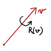
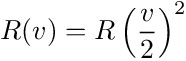
A rotation vector v produces a rotation matrix R(v) by means of a matrix exponential:
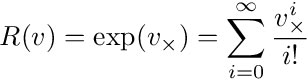
where

is the cross product matrix of v. The exponential is an abstract way of describing how a rotation matrix is formed from a vector, but there is a practical formula called the Rodrigues’ formula:

Rodrigues’ Formula
which can be derived as a consequence of properties of vector cross-products. The Rodrigues’ formula leads to a computational implementation but we need to carefully navigate around a few pitfalls when it comes to using floating point arithmetic:
- Potential divisions by zero. When a is 0 we obviously have a division by zero, but that’s not the end of the story: we can have a non-zero a such that a² is zero in floating point arithmetic.
- Subtractive cancellation. For a close to zero, the last term involves a difference of values close to 1, which causes a loss of significant digits in floating point arithmetic. For example naively evaluating the last term’s coefficient at a=0.1 produces a result that has an error of 40 ulps.
- Poor performance. The naïve evaluation requires the computation of three transcendental functions: square root, sine and cosine, and of an inverse, which might not be that bad but is totally unnecessary for what we want to do.
The first pitfall appears not to be a big deal: after all the graphs of both

look like they could be defined to meaningful values at 0, as the limits as a approaches 0 exists:
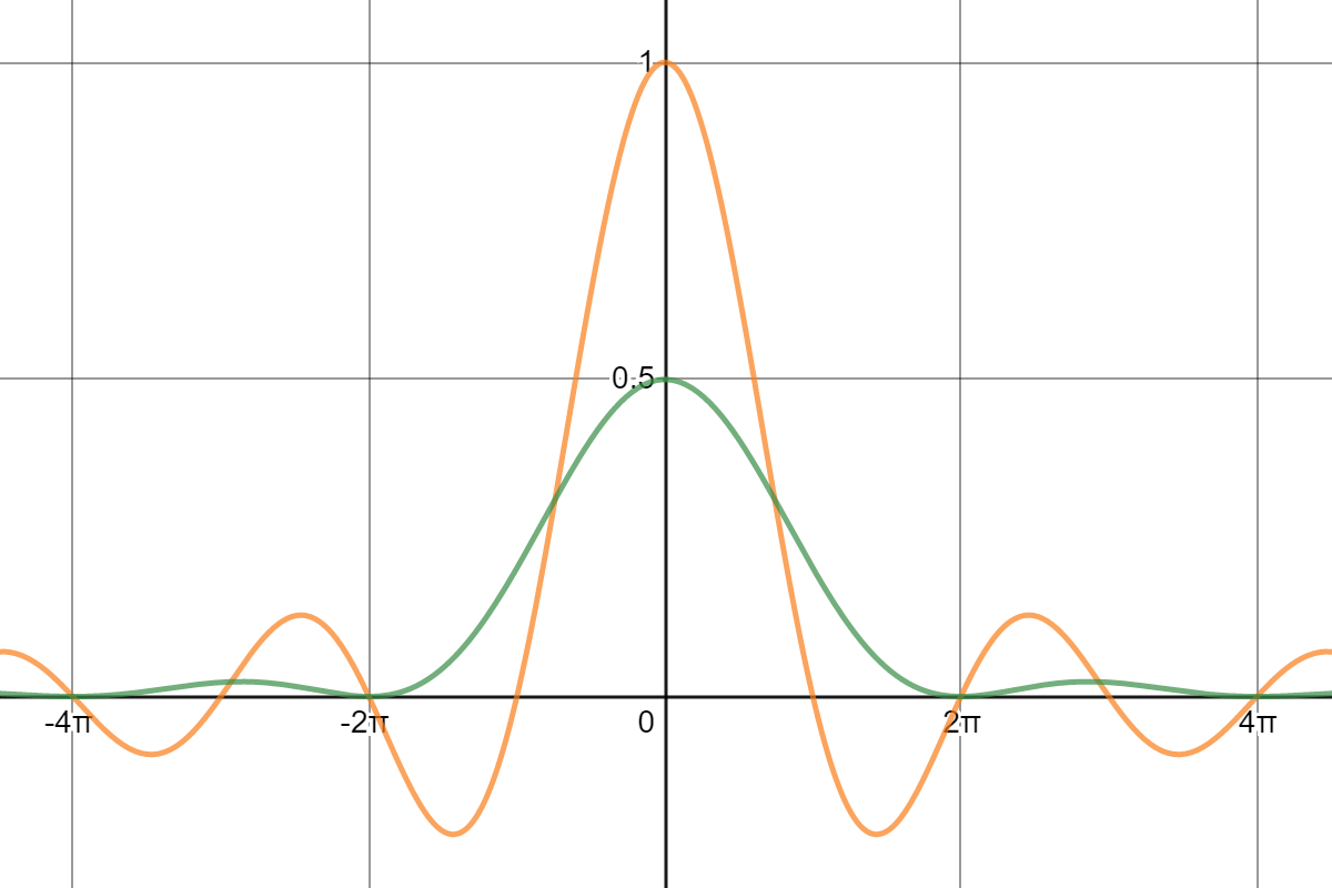
Graphs of S₁ (yellow) and S₂ (green)
These limits are 1 and 0.5 respectively, but instead of redefining the values of these functions exclusively at 0, we can do better and navigate around the other two pitfalls at the same time: the key is to use a Taylor polynomial approximation for both expressions:
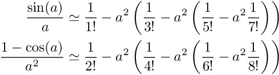
Polynomial approximations of S₁ and S₂
We arranged the terms in a way that will help the implementation to minimize the loss of precision in floating point arithmetic by summing the terms in increasing order of magnitude. Obviously these polynomial approximations are accurate only when a is close to 0. In fact, if we use 32 bit precision, these 6th degree polynomial approximations produce an error that is no more than 1 ulp in the range from 0 to 0.5~π/6 radians.
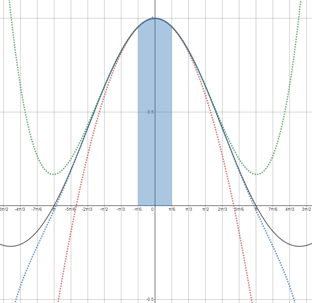
polynomial approximations of S₁. Red: degree 2, Green: degree 4, Blue: degree 6.
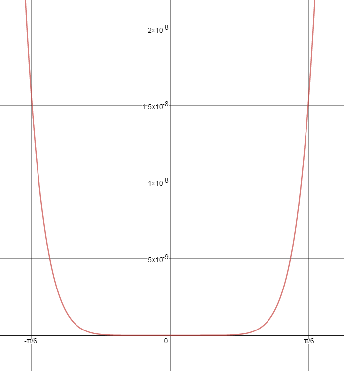
error of the 6th degree approximation.
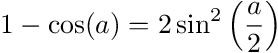
This is great because in that range our estimate is almost as good as it can be and it involves only even powers of a, which removes the need for a square root in the computation of the magnitude of v. For angles above 0.5 but below 1 we can still avoid the transcendental functions by using the “double angle” identity:
which just says that composing two rotation by an angle a/2 is the same as a single rotation by the angle a, and algebraically this follows from the exponential definition of R. We could continue using the above identity for higher angles but at some point doing the explicit computation will just be cheaper. And when doing so we should use the following trigonometric identity to reduce precision loss due to the subtractive cancellation:
The code for computing a rotation matrix from a rotation vector looks like this:
3. Derivative of the Exponential
In previous section we built the function R that maps rotation vectors to rotation matrices:
![]()
A derivative of a function is a linear map that takes infinitesimal variation in the parameters and produces the infinitesimal variation in the result.
The derivative relates small variations in vector v to small variations in rotation matrix R(v)

The derivative relates small variations in vector v to small variations in rotation matrix R(v)
Taking a derivative of R is as simple as taking the partial derivative of each component of R(v) with respect to each component of the vector v. But since a matrix has 9 components and a vector has 3, this results in 27 partial derivatives (it’s a 3rd order tensor, like a matrix but in 3 dimensions)… This is clearly unworkable and we need a better way.
We can reduce the problem to something more manageable: a matrix R is uniquely determined by its action on vectors, that is if we know the result of the matrix-vector product RX for any vectors X, this uniquely determines R as a matrix. So for a fixed vector X we define a function:
![]()
which is a vector valued function of 3 variables. The derivative of F is a matrix (of 9 partial derivatives) and it is called the Jacobian of F:
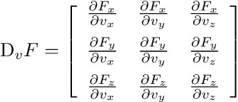
We should not try to compute each entry of this matrix explicitly. This would demand legendary algebraic skills. Instead there is an expression for the Jacobian as a product of two matrices (see this document for details):
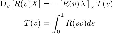
where T(v) is a matrix that depends on v, given by a single parameter integral. First of all, it’s super weird and cool that we have an integral inside a formula for a derivative, but also it is useful to derive properties of the new construct. Also this gives us some intuition about T(v). The effect of applying the matrix T(v) to a vector is to average its orientations by all rotation vectors from 0 to v. Here are some properties that will be useful later:
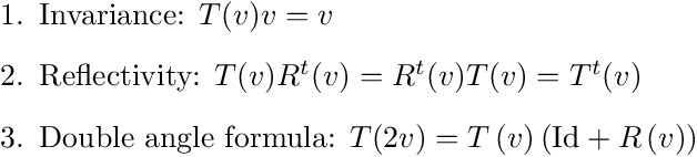
To get a computational method, we simply integrate the Rodrigues’ formula for R(sv):

Formula for T
Like with the formula for R(v), a floating point implementation needs to carefully navigate around similar pitfalls. Both coefficient have limits as a approaches 0:
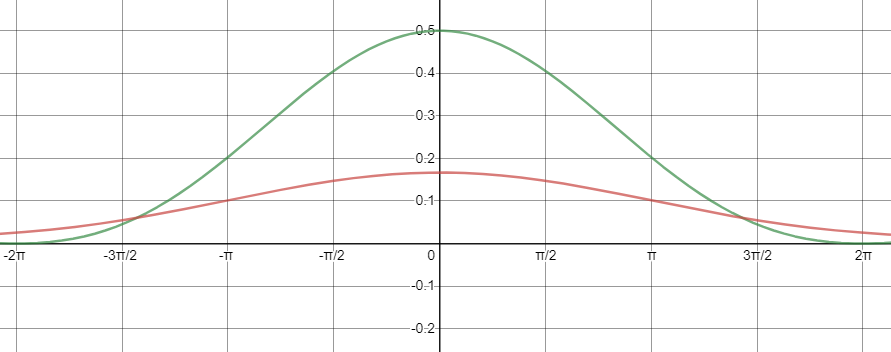
Plots of S₂ and S₃
And again we use Taylor polynomial approximations:
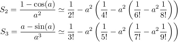
Polynomial approximations of S₂ and S₃
Both degree 6 polynomials are accurate to within 1 ulp for angles up to 0.5 radians. Above 0.5 and up to 1 radians we use the double angle formula to reduce the computation to a smaller angle. And for angles above 1 radians we do the full explicit computation.
The actual implementation will compute both R(v) and T(v) at the same time as they both share a lot of intermediate computations, it allows the use of the double angle formula, and we’ll always use them together anyway.
4. Angular Velocity in Terms of the Rotation Vector
To relate what we derived so far to physics, we need to re-interpret angular velocities in terms of rotation vectors and their time derivatives.
Suppose v(t) is a vector valued function of time t, that describes a path in the 3 dimensional space of rotation vectors. By taking the exponential of its cross-product matrix we get a path in the space of rotation matrices:
![]()
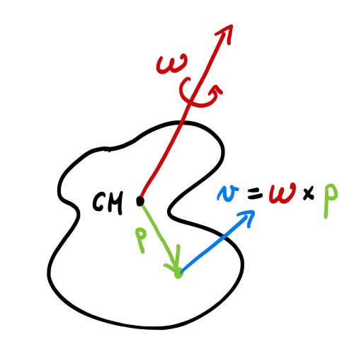
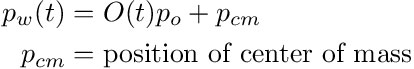
If we pick a point pₒ on the rigid body in local coordinates relative to the center of mass, its motion in world space is described by:
The velocity of this point, which is the derivative of its position with respect to time, is computed using the chain rule of differentiation and the formula for the differential of R from Section 3:

and this gives us a formula for the angular velocity of the rigid body in terms of the rotation vector and its time derivative:
![]()
5. Angular Momentum
The angular momentum of a rotating rigid body is defined as the product of its inertia matrix in world space by its angular velocity. If O is the orientation matrix of the rigid body, the angular momentum is then:
![]()
where the inertia I is in a frame of reference of the moving body. It’s a symmetric matrix (with positive eigenvalues) representing the distribution of mass around the body’s center of mass, and it is constant (in body coordinates). Why is angular momentum important? It’s because the angular momentum doesn’t change unless there are forces applied on the body. Usually this principle is used in the differential form: requiring the time derivative of the angular momentum to be equal to the torque (Angular Momentum and Torque):

In particular, when there is no torque, the angular momentum doesn’t change but the angular velocity can as the world space inertia depends on the orientation matrix O that varies with time… This can make everyone’s head to spin! But there is one constant in nature: the energy. For angular motion, it is:
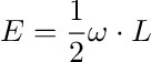
which means that even though ω is non-constant, its projection onto the axis of the angular momentum is, and the graph of angular velocities lies in a plane perpendicular to L, the plane of constant energy. Such a graph is called a herpolhode.
Deviations of the angular velocity from the constant energy plane can be used as a measure of accuracy of a numerical method.
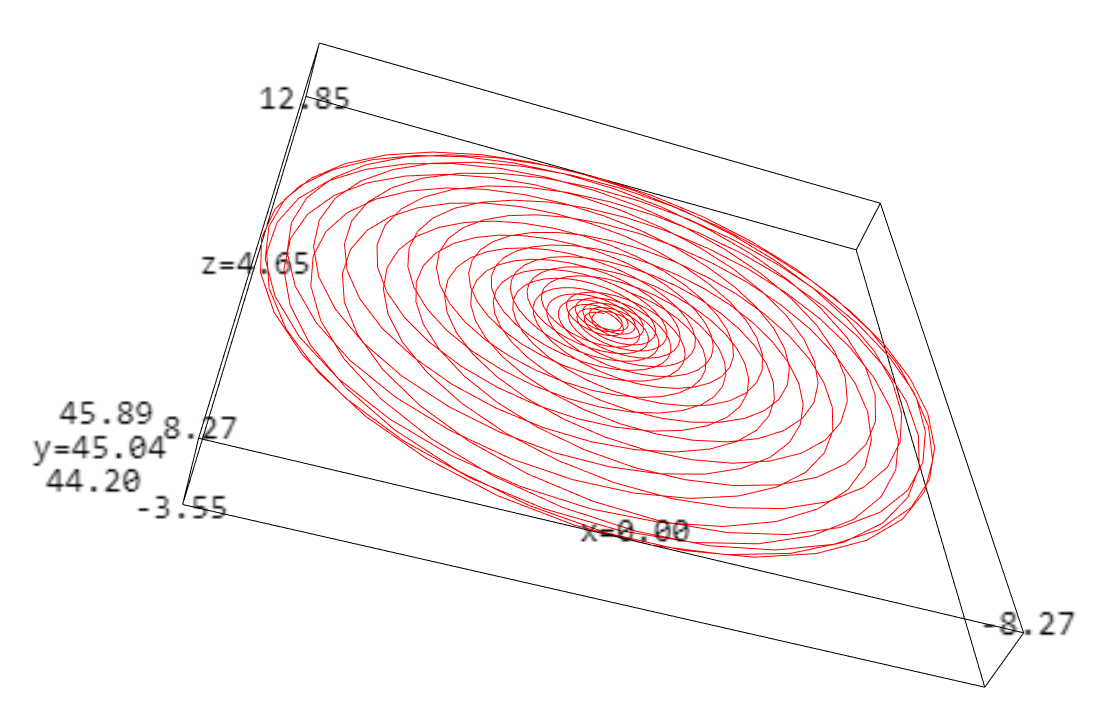
A herpolhode of a body rotating about its intermediate principal axis. It’s the path of the angular velocity vector in world space. Click for the interactive graph.

The body used to generate the above herpolhode
6. Differential Equation of a Freely Rotating Rigid Body
Let’s find the motion of a freely rotating rigid body, without the influence of any torque. The heart of the problem is finding a suitable path v(t) in the space of rotation vectors such that
![]()
is the orientation of the rigid body at any time t. The requirement is that the angular momentum doesn’t change. Using the definition of angular momentum from Section 5, and the formula for the angular velocity from Section 4, we can write the angular momentum in terms of the rotation vector and its derivative:
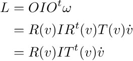
where we used the property of reflectivity of T (see Section 3). We can assume that v(0) = 0 by rotating the world frame to correspond with the orientation of the rigid body at time 0. We can now isolate the derivative of the rotation vector in the last equation to get the first order initial value problem:

The benefits of using the rotation vectors is now clear: it allows to formulate the law of conservation of momentum as a first order differential equation of 3 variables (the three components of v) without requiring any further algebraic constraints between these variables. We now have a clear path to solving the rotational motion by using a standard numerical method for an initial value problem.
For a constant angular momentum L, the above differential equation gives rise to a vector field: for each rotation vector v, we have its time derivative. We can draw this vector field on a ball of radius π, and even animate its flow.
Vector flow of the rigid body differential equation in exponential coordinates. Rotational energy is mapped to hue: low energy in red and high energy in blue.
It’s very interesting to notice that different energy levels form distinct bands. These correspond to angular velocities aligned and counter-aligned with the smallest principal axis (high energy), with the largest principal axis (low energy), and with the intermediate principal axis (green). The low and high energy bands have both two components, which correspond to the two “spins”: momentum is aligned or counter-aligned with the principal axis. The green band is a single component because the rotations around the intermediate principal axis are unstable (Dzhanibekov effect) and fluctuate between the two “spins”.


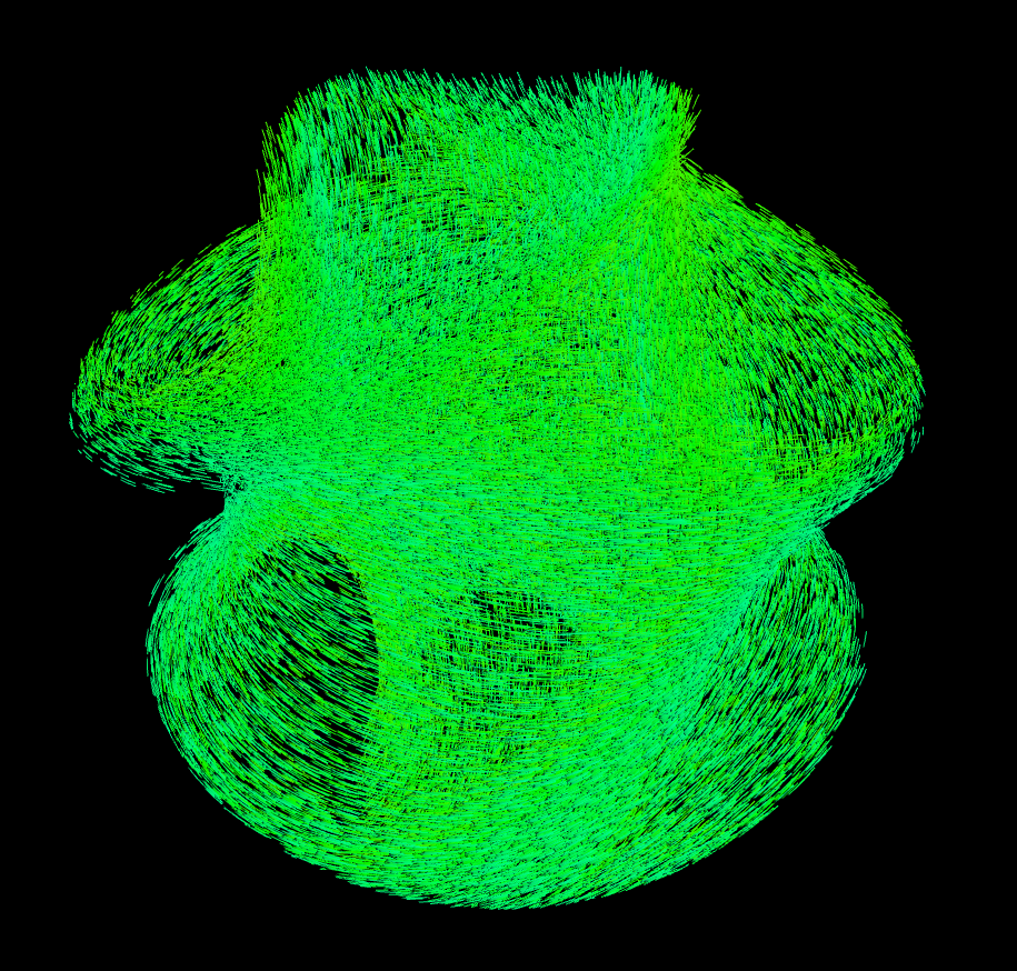
Vector fields of high energy (blue), low energy (red), intermediate energy (green)
7. Implicit Midpoint and Other Methods
Since it’s not always possible to analytically solve a non-linear differential equation like the one above, scientists have developed numerical methods to find approximate solutions. Typically, in games, the simple Euler method is used, which is good enough for most cases but it doesn’t preserve angular momentum. Why is this a problem? Because of behavior like this:

Dancing Lamppost
Notice how the lamppost keeps spinning. This is not a realistic behavior, in reality it should fall flat to the ground releasing its energy in the process. The issue with Euler integration is deeper: bad behavior persists even if we reduce the time steps, the Euler integration ignores non-linear behaviors that are so important in rotational motion.

Idea of a midpoint method
The Implicit Midpoint Method is the simplest integrator (in the Runge-Kutta family) that takes into account non-linear behaviors: it takes into account order 2 terms. It is an integration method with a good energy conservation property at large time scales (technically it’s because it is a symplectic integrator). Although it doesn’t exactly preserve the energy, the energy fluctuates around a constant value and these fluctuations are relatively small. Also this integrator is symmetric under time reversal, which means that if you simulate forward in time and then backward in time, you will get back to the initial conditions, which is great to have for rigid body simulation.
The idea is to approximate the change in the value of the variables over a time step δt by the the derivative at the midpoint between the old and the new value. The “implicit” part of the name comes from the fact that we use the unknown value of the variables to form an implicit expression for this value. Applying this to our differential equation from Section 6, we get the following implicit equation for the rotation vector:
![]()
and because v is invariant under multiplication by T(v), this simplifies to
![]()
Implicit Midpoint Equation
So here we have an expression for v that contains v inside a non-linear term on the right side making it very hard or impossible to isolate v from this equation. The right tool for this job is the Newton’s method for root finding, that we will apply in the next section.
To get an intuition about this equation, let’s divide both sides by δt, and note that the right hand side becomes the angular velocity, in body space, at the midpoint:
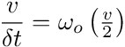
that is the rate of change of the rotation vector is the angular velocity at the midpoint, which seems like a reasonable approximation.
The interesting story here is that it’s now easy to generate other integrators. For example:
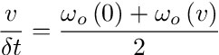
is an integrator that doesn’t come from a standard method as far as I know, but has much better energy conservation properties. I call it the Object Space Trapezoidal Rule (since I noticed this integrator after I began the article, I’m not able to write about it here, but you can derive its implementation using similar math). It does look like the Trapezoidal Rule, though it is not. The actual Trapezoidal Rule is:
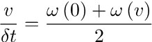
(where angular velocities are in world space) and it has similar energy conservation properties to the Implicit Midpoint, but its Newton’s iteration has a much larger convergence region. This is the method Roblox uses.
8. Newton’s Method
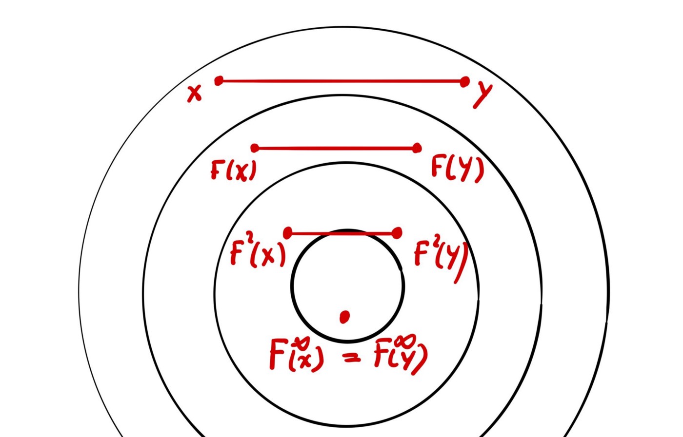
A contraction brings points closer. This process converges to a single point (under some conditions).
We are going to solve our implicit equation by iteratively applying a contraction mapping. A contraction is a function that brings any two values closer to each other in some metric. A property of such a function is that it has a fixed point and that successive iterations converge to such a fixed point. For example to solve the equation of Implicit Midpoint Method from Section 7, we could directly use that equation as the iterator:
![]()
Simple Iterator
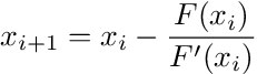
Under some conditions on both I and L, this will converge, but it converges very slowly. The Newton’s method is a way to accelerate such a process. Recall that for an equation of a single variable
![]()
The Newton’s method is the iterative process:
It’s really cool that this method works pretty much the same in higher dimensions. We need to replace the derivative by the Jacobian matrix, and the division by a matrix inverse. So a single Newton’s iteration applied to the Implicit Midpoint equation is:
![]()
Newton’s Iterator
where the Jacobian J is the differential with respect to v:
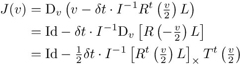
where we used the formula for the derivative of R from Section 3.
Let’s now compare the convergence of the Simple Iterator with the Newton’s Iterator.

Rigid body model used
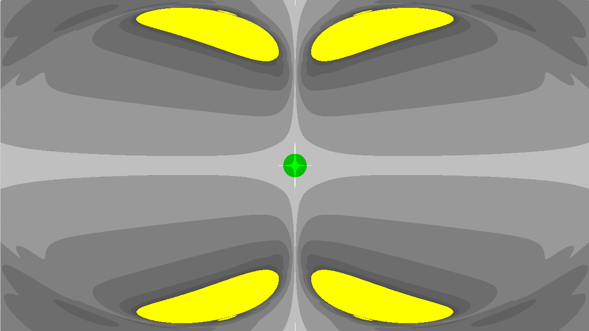
Let’s take this simple model of a rigid body, whose principal moments of inertia are (2.5, 1.4, 1.3). We run the two iterative methods for different values of angular momentum L, and draw a pixel with a shade of grey for the number of iterations it took to reach a certain fixed precision or draw a yellow pixel if it didn’t converge after 10 iterations. The values for L are in the range (-15, -15, 0) to (15, 15, 0) in the xy-plane. The images below were generated by running the algorithms inside a shader.
The image on the left is the result of running the Simple Iteration: the algorithm doesn’t seem to converge except for a small area of values close to the origin. The image on the right shows the results of the Newton’s Iteration. It converges for most of the values and converges much faster. There are still areas of non-convergence and we will need to deal with them, but that’s for a later section.


Convergence map of Simple Iterator (top) and Newton’s Iterator (bottom). Yellow color indicates location where the method doesn’t converge. Shades of gray indicate the number of iterations to achieve some accuracy. Click images for Shadertoy sources.
9. Implementation
We now have almost all elements to implement the Newton’s Iteration for the Implicit Midpoint Method. The question of convergence will be taken care of in the next section. This first function takes as input the inertia matrix and angular momentum and produces the rotation that the body experiences in the time step. The reason we’re not passing the time step as an argument, is because we can assume it to be 1, by pre-multiplying it into L.
The next snippet contains the glue code that calls the solver and properly updates the body orientation:
10. Convergence of the Newton’s Method and Adaptive Sub-Stepping
So we already saw that the Newton’s method doesn’t necessarily converge, and it could return undefined results when the Jacobian becomes non-invertible. Fortunately there is a theorem (of Kantorovich) that provides conditions under which the sequence defined by the Newton’s iterates converge to a solution. If we are looking for zeros of a function F, these conditions are on:
- Starting point of the iteration
- The first and second derivative of the function F
There are many different ways to satisfy these conditions, but we will use a simple method that gives very strict conditions. Using the starting point v=0, the resulting conditions lead to an inequality involving the time-step, inertia and angular momentum (see this document for details):
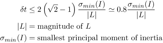
It is not surprising that the time step must get smaller as the momentum increases; what is surprising is the relationship with the smallest principal moment of inertia: for the same angular velocity, bodies with more asymmetric distribution of mass require smaller time steps compared to symmetric ones. The more symmetric the body is, the closer the principal moments of its inertia are, and L~σ(I)ω, and the time step becomes bounded only by the inverse magnitude of angular velocity (times a constant).
As you can see on the image below, the convergence area on the angular momentum graph is rather conservative (green area in the middle). This leads to an adaptive method that does more sub-steps than necessary. With more work, and better choice of conditions for the theorem of Kantorovich, you can enlarge the convergence area and reduce the number of sub-steps necessary.
The green area is where we have mathematical guarantees of convergence.
Another useful piece of information we gain is a bound on the iterates: all the Newton’s iterates vᵢ have magnitudes less than
![]()
which could be useful if we want to simplify the implementations of the function R and T.
The final integration method subdivides the time step into safe sub-steps. At each sub-step it advances by the maximum safe time that respects the convergence condition, and repeats until the entire time step is consumed.
Notice that we used an ortho-normalize to minimize the numerical drift in the rotation matrix. This drift is only due to floating point round off errors in the matrix multiplies and would not be required in infinite precision arithmetic.
11. Measuring Truncation Errors
We use the dancing T-handle again as our prototype body, as it displays the dramatic Dzhanibekov effect when rotating around its intermediate principal axis.
The first pictures shows the energy change as a result of truncation errors of the integration method. The x and y axes correspond to different values of angular momentum in the z=0 plane, in the range from about (-50, -50, 0) to (50, 50, 0). The inertia matrix is diagonal with principal moments (2.5, 1.4, 1.3). The lighter/darker areas represent larger/smaller relative energy differences, with the largest value being around 0.3%. The relative error stays bounded as angular momentum (or time step) increases, which means the simulation doesn’t gain or lose energy at large time scales.

Energy change due to truncation error of the integration method
The way to read this picture is to look at straight rays starting at the origin as the evolution of the state of a rotating body, walking outwards as time flows forward. This is because simulating a body with angular momentum L over some time Dt is the same thing as simulating the same body but with momentum Dt L over the time 1. So walking a ray, which increases the magnitude of L, is equivalent to increasing the time step of the simulation.
For the Object Space Trapezoidal Rule (see Section 7), the energy fluctuations are dramatically smaller (under 10^-5 of the magnitude), but the convergence area of the Newton’s iteration is very small. The actual Trapezoidal Rule has similar energy fluctuations to the Implicit Midpoint, but has a much larger convergence area.
12. Application to the Dancing Pole

Euler’s Method.

Implicit Midpoint. No gravity.
We can now simulate the spinning pole we first encountered in the introduction. Let’s turn off gravity to observe what happens. Where with the Euler method, the pole continues spinning around its vertical axis (close to the smallest principal axis), with the new method the pole acquires a secondary precession spin around a large principal axis. In presence of gravity, this precession spin would cause the pole to fall flat to the ground.
— — —
Maciej Mizerski is a Technical Director at Roblox that specializes in mathematical simulation and optimization. With more than 10 years in the games industry and a doctorate in mathematics, he holds a deep understanding of mathematical methods, physics simulation, optimization and cross platform development. Previously at Relic Entertainment and Radical Entertainment.
Neither Roblox Corporation nor this blog endorses or supports any company or service. Also, no guarantees or promises are made regarding the accuracy, reliability or completeness of the information contained in this blog.
©2020 Roblox Corporation. Roblox, the Roblox logo and Powering Imagination are among our registered and unregistered trademarks in the U.S. and other countries.