Deep learning has been drastically changing the field of machine learning (and the world accordingly) as machine learning has been much more widely applied now to different application scenarios – such as recommender systems, speech recognition, autonomous driving, and automatic game-playing. In 2018, Professor Joshua Bengio, Geoffrey Hinton, and Yann Lecun received the Turing award (often referred to as the “Nobel Prize of Computing”) for their contributions to deep learning. However, deep learning is still viewed as a black box by many researchers and practitioners, and theoretical explanations on the mechanism behind it are still well expected. So let’s explore why the basic principle behind deep learning is quite generic via the relationships between the state-of-the-art deep learning models and several early models not under the deep learning title (including a model co-invented by myself).
Neural networks can be interpreted as either function-universal approximators or information processors. We will try to explain the mechanism of deep learning from the perspective of function-universal approximators. Function-universal approximation has been a traditional topic and we will review a few neural networks prior to and in the era of deep learning. Through their similarities and differences, we will show why neural networks need to go deep and how deep they actually need to be. And our theory coincides with the convolutional neural networks currently in use very well.
Traditional Neural Networks
There has been a long history of neural network models. And its activation function is typically a sigmoidal function or a hyperbolic tangent function. Neural networks with multiple layers were named multi-layer perceptron (MLP) [1]. And it could be trained by the backpropagation method proposed by David Rumelhart, Geoffrey Hinton, and Ronald Williams in 1986, which is essentially a gradient-based method. These activation functions are nonlinear and smooth. Also they have bell-shaped first derivatives and fixed ranges. For example, sigmoidal function pushes the output value towards either 0 or 1 quickly, while hyperbolic tangent function pushes the output value towards either -1 or 1 quickly. These make them well-suited for classification problems. However, as the number of layers increases, the gradients start vanishing due to the employment of the backpropagation method. So MLP models with one hidden layer were possibly the ones most commonly seen then.
Also, it is widely known that Rectified Linear Unit (ReLU) has been used as the activation function in deep learning models in replacement of the sigmoidal and hyperbolic tangent functions. Its mathematical form is as simple as max{0, x}, and it has another name ramp function. The reason for using it is its gradient slope with respect to x is 1, so the gradient will never vanish as the number of layers increases. Let us look at deep neural networks from the perspective of ReLU further.
Continuous Piecewise Linear Functions
One of the earliest models using ReLU for regression and classification was the hinging hyperplanes models proposed by Leo Breiman in 1993 [2]. Professor Breiman was a pioneer in machine learning and his works greatly bridge the fields of statistics and computer science. The model is the sum of a series of hinges so it could be viewed as a basis function model like B-spline and wavelet models. Each hinge in his model is actually a maximum or minimum function of two linear functions. This model can be used for both regression and classification. A binary classification problem can be viewed directly as a regression problem, while a multi-class classification problem can be viewed as multiple regression problems.
The model proposed by Breiman can be viewed as one-dimensional continuous piecewise linear (CPWL) functions. Shunning Wang proved in 2004 that this model can represent arbitrary continuous piecewise linear functions in one dimension and nesting of such kinds of models is needed for representation of arbitrary CPWL functions with multi-dimensional inputs [3]. Based on this theoretical result, Ian Goodfellow proposed a deep ReLU neural network named Maxout networks in 2013 [4]. The theoretical basis for using CPWL functions to approximate arbitrary nonlinear functions is just Taylor’s theorem for multivariable functions in Calculus.
Since the 1970s, Leon O. Chua and other researchers have proposed a cellular neural network to represent CPWL functions with inputs in different dimensions [5][6][7]. Professor Leon Chua has made great contributions in the area of Circuits and Systems, and this work has received prestigious awards from the community of neural networks. The need for a more complicated nonlinear component to represent the structure with inputs of two or more dimensions was caused by the linear separability problem widely known in machine learning. In Breiman’s model, all the boundaries are taking place when two linear functions in each hinge are equal, so all the boundaries are linear and effective in the entire domain. So it can not represent CPWL functions with two-dimensional inputs such as the example shown in Figure 1 [8].
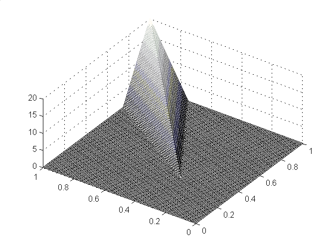
Figure 1. A CPWL function with a two-dimensional input
Chua’s model chose to use nested absolute functions to build the nonlinear components of the model, and the level of nesting is equal to the dimension of the input. So this model may have a lot of parameters when the input dimension is high.
In 2005, Shunning Wang and Xusheng Sun generalized the hinging hyperplane model to arbitrary dimensions [8]. They have proven that any CPWL functions can be represented by the sum of the maximum or minimum functions of at most N + 1 linear functions, where N is the dimension of the input. They have also pointed out that this is equivalent to a deep neural network with two features: first, the ramp function is used as the activation function; second, the maximum number of layers is the ceiling of log2(N+1), where N is the dimension of the input. This greatly reduced the theoretical bound on the number of layers. And generally this model can be trained using gradient-based methods. In the past decade or so, there are many works done in the area of algorithm and architecture to make the training better and easier.
Deep Learning Models
One of the big milestones in the history of deep learning is AlexNet used in an ImageNet competition in 2012 [9]. Alex Krizhevsky, Ilya Sutskever, and Geoffrey Hinton proposed a deep neural network model that consists of 8 convolutional or dense layers and a few max pooling layers. The network achieved a top-5 test error of 15.3%, more than 10.8 percentage points lower than that of the runner-up. Its input is of 224 * 224 in each of the RGB channels, so its total dimension is 224 * 224 * 3. Then our bound on the depth of the neural network is 18. So if the bound is meaningful, deeper neural networks would be possible to make the accuracy higher. Karen Simonyan and Andrew Zisserman proposed the VGG model in 2014 [10]. It has typical variants with 16 or 19 convolutional or dense layers, and further improved the accuracy as expected. This coincides with our theory well and there is at least one more thing that can be done to possibly even further increase the accuracy in some cases.
In both AlexNet and VGG, the depth of the subnet ending at each activation function is identical. Actually, we only need to guarantee that enough number of components in the networks is of no less depth than the bound. In other words, the number of the linear functions in each maximum or minimum function in the generalized hinging hyperplane model could be flexible in practice. And it could be more parameter efficient to have some components with an even larger depth and some components with a smaller depth. Kaiming He, Xiangyu Zhang, Shaoqing Ren, and Jian Sun proposed the ResNet model in 2015 [11]. This model chose to let some components bypass some previous layers. Generally this model is deeper and narrower and has some variant of as deep as 152 layers, and improved the accuracy even further.
We have been focusing on convolutional neural networks in this article. Other deep neural networks such as recurrent neural networks need to be explained by other theories. Also, there are still new innovations in the area of activation functions such as exponential linear unit (ELU) [12]. In my opinion, modeling & training algorithms, data availability, computational infrastructure, and application scenarios together have made the wide application of deep learning nowadays.
References:
[1] D. E. Rumelhart, G. E. Hinton, and R. J. Williams (1986) Learning representations by back-propagating errors. Nature, 323, 533–536.
[2] L. Breiman, “Hinging hyperplanes for regression, classification, and function approximation,” IEEE Trans. Inf. Theory, vol. 39, no. 3, pp. 999–1013, May 1993.
[3] S. Wang, “General constructive representations for continuous piecewise-linear functions,” IEEE Trans. Circuits Syst. I, Reg. Papers, vol.51, no. 9, pp. 1889–1896, Sep. 2004.
[4] I. J. Goodfellow, D. Warde-Farley, M. Mirza, A. Courville and Y. Bengio. “Maxout Networks,” ICML, 2013.
[5] L. O. Chua and S. M. Kang, “Section-wise piecewise-linear functions: Canonical representation, properties, and applications,” IEEE Trans. Circuits Syst., vol. CAS-30, no. 3, pp. 125–140, Mar. 1977.
[6] L. O. Chua and A. C. Deng, “Canonical piecewise-linear representation,” IEEE Trans. Circuits Syst., vol. 35, no. 1, pp. 101–111, Jan. 1988.
[7] J. Lin and R. Unbehauen, “Canonical piecewise-linear networks,” IEEE Trans. Neural Netw., vol. 6, no. 1, pp. 43–50, Jan. 1995.
[8] S. Wang and X. Sun, “Generalization of hinging hyperplanes,” in IEEE Transactions on Inf. Theory, vol. 51, no. 12, pp. 4425-4431, Dec. 2005.
[9] A. Krizhevsky, I. Sutskever, and G. Hinton. Imagenet classification with deep convolutional neural networks. NIPS, 2012.
[10] K. Simonyan and A. Zisserman. “Very deep convolutional networks for large-scale image recognition,” ICLR, 2015.
[11] K. He, X. Zhang, S. Ren, and J. Sun. Deep residual learning for image recognition. CVPR, 2015.
[12] D.-A. Clevert, T. Unterthiner, and S. Hochreiter, “Fast and accurate deep network learning by exponential linear units (ELUS),” ICLR, 2016.
Neither Roblox Corporation nor this blog endorses or supports any company or service. Also, no guarantees or promises are made regarding the accuracy, reliability or completeness of the information contained in this blog.
This blog post was originally published on the Roblox Tech Blog.