Let’s build our own state-of-the-art, multiscattering, GGX BRDF (bidirectional reflectance distribution function) for physically based rendering.
Of course, this has all been built before – by very smart people who used their knowledge of math and physics to create sophisticated solutions. If you wanted to do a whole lot of reading to achieve a similar result, feel free to try these great articles:
- Stephen Hill – “A Multifaceted Exploration”
- Danny Chan “Material advances in Call of Duty: WWII”
- McAuley “A journey through implementing Multiscattering BRDFs and Area Lights”
But we’re going to skip all that reading and do things the easy way. Ready?
Let’s start from your vanilla contemporary GGX with all the correlated-Smith fixings. The following sequence of images is generated with Disney’s BRDF explorer environment lighting mode. It shows a metallic GGX with varying roughness, from 0.3 to 0.9, using the common parametrization of alpha = roughness squared.

Notice how the material looks too dark at high roughness. Once again, smart people have worked hard to find and fix this issue.
Let’s compare the image above with Kulla/Conty’s Multiscattering GGX BRDF.

Fixed!
Now, we could try to work out how this solution works. The math is already there, and you probably should. It’s both interesting and useful for understanding other related problems. But remember, we’re going to skip all that here.
Let’s start at the top. Why do we prefer PBR (physically based rendering)? It’s not because we like physics (at least, I don’t). And if we were deeply concerned about physics, this would be a small error to focus on considering that we are surely committing worse sins in our end-to-end image pipeline…
Computer graphics isn’t predictive rendering. We aren’t simulating physics for realism, that’s not the goal. We’re trying to make pretty pictures.
We noticed that simulating some physics to make pretty pictures allowed for easier workflows: decoupling materials from lighting, reducing the number of hacks and parameters, allowing to use libraries of real materials, and so on.
So when making decisions about how to proceed, we have to consider the artistic concerns ahead of the technical ones. If there’s an artistic problem we can identify, then we can look to physics to see if there’s a technical solution. In our current BRDF, the problem is that it would be nice if our material parameters were orthogonal, and having things get darker as we change roughness is not ideal.
So then, can physics help? Is this darkening physically correct, or not? How do we test? Enter the furnace! Let’s put our GGX-coated metallic object in a uniformly lit environment and see what happens:

Light hits our surface, and hits our microfacets. The microfacets reflect back some light, and refract some, according to Fresnel. If we’re assuming this surface is metal, physics tells us that the refracted light, that which goes “inside” the surface, gets absorbed and never comes out (as it is converted into heat).
It’s reasonable that even in a furnace our metallic object has a color, as some of the energy will be absorbed. But what if we take our microfacets and make them always reflect all the light, no absorption?
This means we need to set our f0 to 1 (remember, Fresnel is what controls how much light the microfacets scatter). Let’s try that and see what happens:

The object is still not white. Something’s wrong! Now, an inquisitive reader might say, “How do you know it’s wrong? Perhaps certain directions scatter more light and others less?” It’s not always easy to intuit the correct solution.
Let’s instead consider what a light path, starting from the camera, looks like. It will hit one or many of the microfacets, bounce around, then eventually escape and connect to the furnace environment – which will always be emitting a given constant energy.
So how much of that energy should reach the camera? All of it! Because based on our setting, all the energy should be reflected no matter how many microfacets it hits. All light paths lead to the camera, eventually.
So that’s why the image above should be completely white. Since it isn’t, we must have a problem in our math.
If you studied BRDFs, you know that in the microfacet model there is a masking-shadowing visibility function that models which microfacets are occluded by others. What we don’t typically model, though, is the fact that these occlusions are themselves microfacets, so the light should bounce around and eventually get out, not discarded.
This is what the multiscattering models model and fix, and if we put Kulla and Conty’s GGX into a furnace, it would generate a totally boring, totally correct white image for a fully reflective material regardless of roughness.
Kulla’s model is not simple though, and in many cases is not worth using for such a minor problem. So, can we be even more simplistic in our solution? What if we knew how much light our BRDF gives out in a furnace, for a given roughness and viewing angle (fixing then again f0=1)? Could we just take that value and normalize the BRDF with it?
Spoiler alert: we can, easily. We already have this “furnace” value in most modern engines in the look-up tables used for the popular split-sum image-based lighting approximation.
The split-sum table boils down the “BRDF in a furnace” (also known as directional albedo or directional-hemispherical reflectance) to a scale and bias (add) factor to be applied to the Fresnel f0 value.
In our case, we want to normalize considering f0=1, so all we do is scale our BRDF lobe by one over bias(roughness,ndotv) + scale(roughness,ndotv). This is the result:

We’re getting some energy back at high roughness, and if we tested this in a furnace it would come up white, correctly, at f0=1. But it’s also different from Kulla’s. In particular, the color is not quite as saturated in the rough materials. How come? Again, if you studied this problem already (cheater!) you know the answer.
Proper multiscattering adds saturation because as light hits more microfacets before escaping the surface, we pick up more color (raising a color by a power results in a more saturated color). So how can this be physically wrong, but still correct in our test?
By not simulating this extra saturation we are still energy-conserving, but we changed the meaning of our BRDF parameters. The “meaning” of f0 in our “ignorant” multiscattering BRDF is not the same as Kulla’s. It results in a different albedo, but the BRDF itself is still energy-conserving. It’s just a different parametrization.
Most importantly, I’d say it’s a better parametrization! Remember our objectives. We don’t do physics for physics’ sake, we do it to help our production.
We prefer to make our parameters more orthogonal so that artists don’t need to artificially “brighten” our BRDF at high roughness. If we go with the “more correct” solution (about that, this recent post by Narkowicz is a great read) we would add a different dependency, so that roughness, instead of darkening our materials, makes them more saturated (which would kind of defeat the purpose). You can imagine some scenarios where this might be desirable, but I’d say it’s almost always wrong for our use-cases.
If we wanted to simulate the added saturation, there are a few easy ways. Again, going for the most “ignorant” (simple) we can just scale the BRDF by 1+f0*(1/(bias(roughness,ndotv) + scale(roughness,ndotv)) – 1), resulting in the following:

Now we’re getting close to Kulla’s solution. If you’re wondering why Kulla’s approximation is better, as it might not show in images, it’s because ours doesn’t respect reciprocity.
That might be important for Sony Imageworks (as certain offline path-tracing light transport algorithms do require it), but it’s fairly irrelevant for us.
So now that we’ve found an approximation we’re happy with, we can (and should) go a step further and see what we’re really doing. Yes, we have a formula, but it depends on some look-up tables.
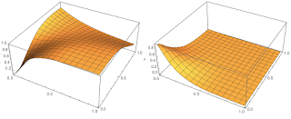
This isn’t a big issue (we need these tables around for image-based lighting anyways), but it would be an extra texture fetch and it’s always important to double-check our math. So let’s visualize the 1/[bias(roughness,ndotv) + scale(roughness,ndotv)] function we’re using:
It looks remarkably simple! In fact, it’s so simple you don’t need a sophisticated tool to find it – so I’ll just show it: 1 + 2*alpha*alpha * ndotv. Very nice.
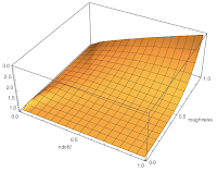
Approximation compared to the correct normalization factor (gray surface)


You can see that there is a bit of error in the furnace test. We could improve it by doing a proper polynomial fit (turns out “2” and “1” in the formula above are not the best constants), but defining what’s “best” would be a problem all on its own, because doing a simple mean-square minimization on the normalization function doesn’t really make a lot of sense (we should care about end visuals, perceptive measures, which angles matter more and so on). We’ve already spent too much time for such a small fix. Moreover, the actual rendered images are really hard to distinguish from the table-based solution.
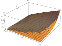
Now let’s see what could we achieve if we wanted to go even simpler by dropping the dependency from ndotv. It turns out, in this case, 1+alpha*alpha does the trick decently as well.
We’re applying a multiplicative factor to our BRDF to brighten it at high roughness, which just makes a lot of sense.
Of course, this adds more error, and it starts to show as the BRDF shape changes. We get more energy at grazing angles on rough surfaces, but it might just be good enough depending on your needs:


Under-exposed to highlight that with the simpler approximation sometimes we lose light, sometimes we add.
Hopefully you’ve figured out the big lesson here. Sure, you can devote yourself to chasing graphics that perfectly simulate real-world physics. But you can also just cheat. And whether it’s for performance, simplicity, or just pure laziness, sometimes cheating is the right answer.
Neither Roblox Corporation nor this blog endorses or supports any company or service. Also, no guarantees or promises are made regarding the accuracy, reliability or completeness of the information contained in this blog.
This blog post was originally published on the Roblox Tech Blog.