How We Scaled Bert To Serve 1+ Billion Daily Requests on CPUs

Here’s a classic chicken-and-egg problem for data scientists and machine learning engineers: when developing a new machine learning model for your business, do you first make it accurate, then worry about making it fast in production? Or do you first make sure it can be fast, then make it accurate? Ask the question and a lively debate always ensues!

In early 2019, we were faced with that exact scenario as we started developing our next-generation text classifiers for Roblox, using (at the time) new bleeding-edge Bert deep learning models. We were unsure if Bert models, which are large deep neural networks whose “entry-level” base model starts at 110 million parameters, could meet our demanding speed and throughput requirements in production. We forged ahead with making our Bert-based text classifiers highly accurate, and in the tense months that followed we fortunately were able to make it fast enough for production. So for us the “chicken” (accuracy) came first, then the “egg” (speed) came after. While this was a stressful experience for us, it doesn’t have to be for you, because in this article we are going to share the optimizations that made Bert inference fast for us. So you can start with an egg (a known playbook for making certain Bert models fast in production), then focus on the chicken (making your Bert model accurate).

Our Journey To Making Bert Fast in Production

The magic of Bert for Natural Language Processing (NLP) was well-chronicled in 2019, and here at Roblox we have seen that magic working up close on our own data. By fine-tuning Bert deep learning models, we have radically transformed many of our Text Classification and Named Entity Recognition (NER) applications, often improving their model performance (F1 scores) by 10 percentage points or more over previous models.

However, while our Bert model development was accelerated by plenty of amazing resources and awesome libraries, we found only a few resources on how to scale Bert on PyTorch for low-latency and high-throughput production use cases. And for many of our NLP services, we needed to handle over 25,000 inferences per second (and over 1 billion inferences per day), at a latency of under 20ms.

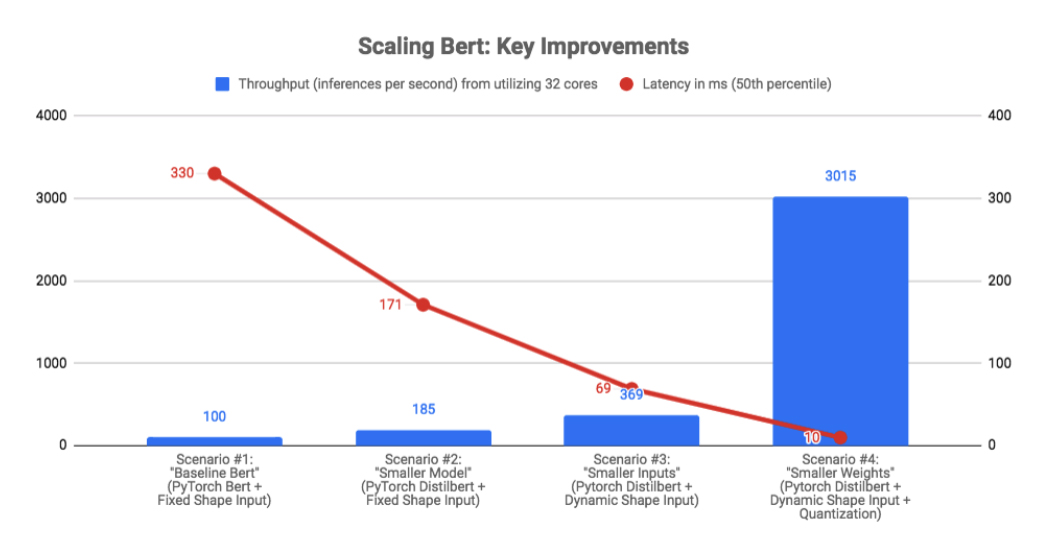
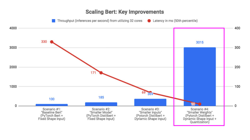
The goal of this article is to share our journey of speeding up Bert inference by over 30x for text classification at Roblox. Through these improvements (summarized below), we were able to not only make Bert fast enough for our users, but also economical enough to run in production at a manageable cost on CPU.

The Benchmark

For the purposes of this article, we will focus on improving the inference speed of a text classification service that was developed by fine-tuning Bert. Here “inference” refers to the chain of taking text as input, tokenizing it into an input tensor, feeding that tensor to our Bert-based model, and returning a classification label produced by the model.

Anytime we seek to systematically improve speed, we must choose a benchmark. The chosen benchmark for our Bert classifier had two components:

• Latency: the median time it takes to serve one inference request (we also have 99th percentile plus benchmarks internally)
• Throughput: the number of inferences we can serve in one second

For consistent throughput comparisons, our benchmark code launched exactly 32 worker processes, which each sequentially ran through 1000 inference requests. This benchmark was run on a single server with 36 Xeon Scalable Processor cores.

This benchmark simulated a production setting where a text classification service was supported by a pool of worker processes. Under load, each worker was busy processing consecutive inference requests for sustained periods of time. In our actual production environment, we had hundreds of these workers across many machines, so that we could support over 25,000 requests per second with median latencies of under 20ms.

Tooling

Our fine-tuned Bert model was developed using the Huggingface Transformers library v2.3.0. We chose Huggingface specifically for its PyTorch support, and we are currently in production with PyTorch 1.4.0. Huggingface made it easy for us to experiment with the many other transformer-based models, including Roberta, XLNet, DistilBert, Albert, and more. It’s the way we discovered DistilBert which improved our inference speed dramatically (we will discuss this in a bit).

First Up: CPU or GPU for Inference?

Our first big decision was whether to run inference for our Bert-based text classifier on CPU or GPU.

For our model training, GPU was undoubtedly much faster than CPU. Fine-tuning (training) our text classification Bert model took over 10x longer on CPU than on GPU, even when comparing a Tesla V100 GPU against a large cost-equivalent 36-core Xeon Scalable CPU-based server.

For inference, the choice between GPU and CPU depends on the application. These are the factors that swung our decision to CPU for inference:

• Simplicity. GPUs scale best when inputs are batched. Our text classifier, however, operates in a real-time request-response setting. Therefore, batching these real-time requests would only create overhead and complexity. Running inference on CPU offered us a simpler path forward, because on CPU our Bert model performed extremely well even when we did not batch its inputs.
• Favorable Cost Economics. For our text classifier, the cost economics of inference on CPU was better than on GPU. After applying all the scaling improvements in this article, throughput for our text classification service was 6x higher per dollar on CPU compared to GPU. Specifically, we could scale our Bert-based services to over 3,000 inferences per second on an Intel Xeon Scalable 36-core server, versus 500 inferences per second on a cost-equivalent Tesla V100 GPU.

CPU Recommendation

For our benchmarking, we found 2nd Generation Intel Xeon Scalable processors worked best due to excellent support for deep learning inference. For example, some of our most impactful speedups leverage Vector Neural Network Instructions and dual Fused-Multiply-Add (FMA) cores featured on 2nd generation Xeon Scalable Processors. All of the results we report in this article are on Intel Xeon Scalable Processor series chips. Your mileage may vary on other CPU configurations, as our testing on different chips has been limited.

Thread Tuning

The first blocker we encountered with scaling Bert inference on CPU was that PyTorch must be properly thread-tuned before multiple worker processes can do concurrent model inference. This was because within each process, the PyTorch model attempted to use multiple cores to handle even a single inference request. Therefore, each process was competing for the same limited resources (physical cores). This resulted in stagnation when too many of these workers were running at once in the same machine.

Fortunately, the remedy to this was simple: in each inference-performing worker process, we simply set the number of threads to 1 as shown in line 9 below.

What was the impact of doing this? When lots of worker processes were running on the same machine, the scaling was more orderly because each worker was only using one core. This is what allowed us to scale to many processes on a single machine, so that we could increase the throughput on each machine while maintaining an acceptable latency.

Scenario #1: Bert Baseline

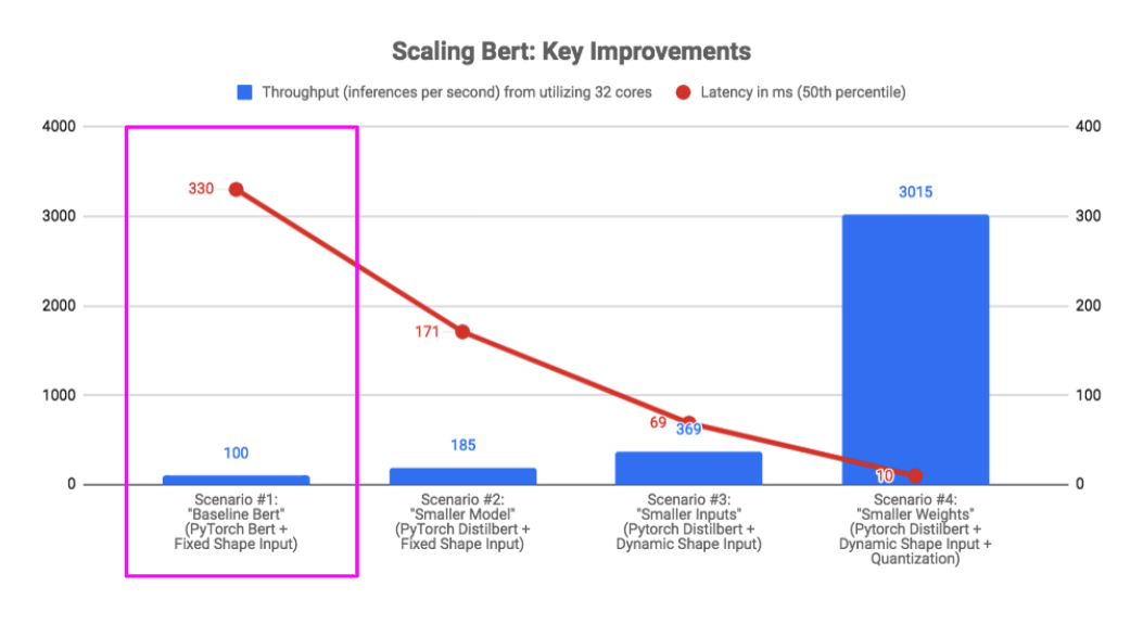
The first baseline was a vanilla Bert model for text classification, or the architecture described in the original Bert paper. This Bert model was created using the BertForSequenceClassication Pytorch model from the Huggingface Transformers 2.3.0 library. In this scenario, we also made one intentionally-naive design choice – we zero-padded all tensor inputs into a fixed length of 128 tokens. The reason for doing this was that zero-padding is required when batching inputs, so that all inputs are the same size. Since it’s easy to accidentally zero-pad the inputs even when the batch size is 1, we wanted to quantify the performance penalty of doing so in this baseline scenario.

In the pink box below, we show the benchmark result for this “Bert Baseline” scenario. Even at 330ms, the latency was too high for our production needs, and the throughput was terrible for the number of cores being utilized by the benchmark.

Scenario #2: Smaller Model (DistilBert)

After Bert was released in October 2018, there have been plenty of models that tried to push forward the state of the art by creating models with more parameters. While Bert base has 110 million parameters, some of these newer models have over 1 billion parameters with marginally higher statistical performance and considerably worse computational performance. What we wanted, however, was better computational performance, and we were willing to sacrifice a little statistical performance to get it.

Luckily for us, in October 2019 Sanh et al introduced DistilBert, one of many models that bucked the trend of larger Bert-like models. These “smaller models” focused on reducing the size of Bert, which led to much faster inference and training, with a minimal loss in statistical performance.

We chose DistilBert for two main reasons. First, DistilBert is roughly twice as fast as Bert, yet its statistical performance (F1 score) on our text classification was within 1% of Bert. Second, the Huggingface Transformers library made it very straightforward for us to swap DistilBert for Bert, allowing us to keep our training and inference pipelines intact.

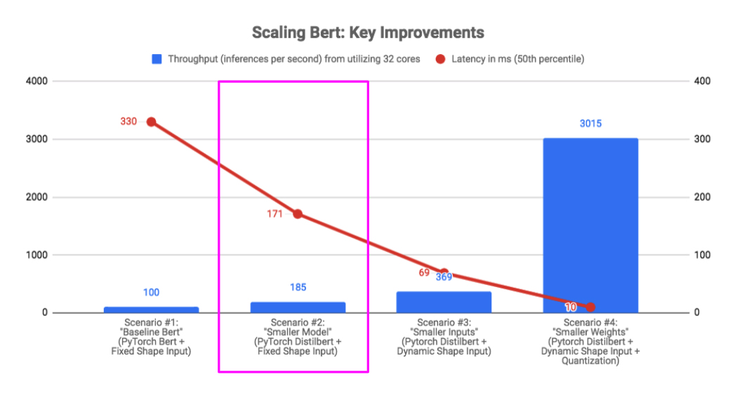
Here was the benchmark result when we used the smaller DistilBert model instead of the larger Bert. As we can see, we almost halved our latency while nearly doubling our throughput.

Scenario #3: Smaller Inputs (Dynamic Shapes)

Our next improvement came from making something else smaller, in this case the tensor inputs to the DistilBert model.

First a little background on zero-padding. A deep learning model generally expects a batch of tensors as input. For our text classifier this means representing textual input as a tensor through Bert tokenization, then batching those tensors. Since text is variable in length, we must also zero pad the resulting variable-length tensors to produce a fixed-shape batch, such shown here:

As mentioned earlier, our text classifier operates in a real-time request-response setting. As such, our ideal batch size is 1. The implication is that we did not need to zero-pad the tensors at all, since all tensors have the same size when the batch size is 1. Here is what the input texts from above looked like when we sent them to the model in separate batches with no zero padding:

We call this “dynamic shapes” since we are allowing variable-length tensors in each batch. Moving to inputs with dynamic shapes greatly improved our throughput and latency. Intuitively, this makes sense because we were making the model inputs smaller by not zero padding. Moreover, there was no negative impact to our F1 scores since our model output probabilities were the same whether we used dynamic shapes or zero padding.

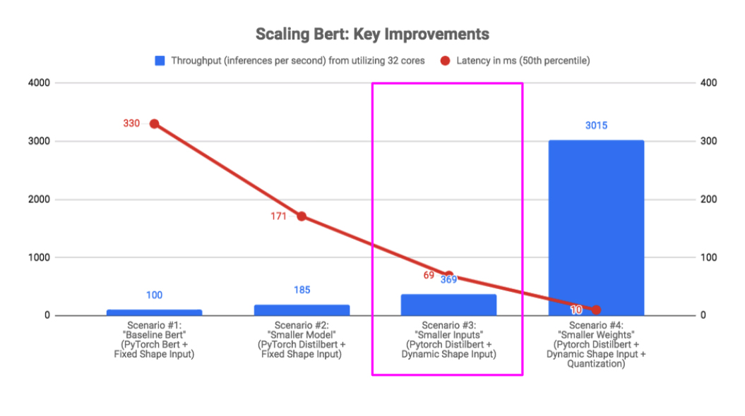
Here was the benchmark result when we used DistilBert + Dynamic Shapes. As we can see, we more than halved our latency while doubling our throughput.

Scenario #4: Smaller Weights (Quantization)

We saw our largest performance boost from smaller weights, achieved through a technique called quantization.

Quantization involves improving the efficiency of deep learning computations through smaller representations of model weights, for example representing 32-bit floating point weights as 8-bit integers. The specific quantization technique we leveraged for our DistilBert model was “Dynamic Quantization”. This technique involves quantizing weights AFTER training, as opposed to quantizing during training (which is called Quantization-Aware Training).

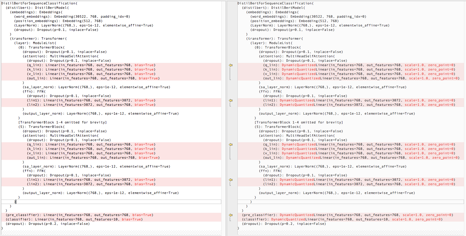
The Dynamic Quantization support in Pytorch 1.3+ was very easy to implement, and a one-line change in our code enabled the use of 8-bit integer representations of weights in all linear layers of the DistilBert model:

Here is a visualization of how this quantization changed the original DistilBert model. As you can see, PyTorch will replace the “Linear” layers such as the attentional Query (Q), Key (K), and Value (V) layers with a “Dynamic Quantized Linear” layer, which will use the quantized 8-bit integers in its internal multiply/add operations.

Here was the benchmark result when we used Distilbert + Dynamic Shapes + Dynamic Quantization. We can see that the effect of all three of these optimizations together creates a very large 30x improvement over our vanilla Bert baseline in both latency and throughput.

We also observed a small negative F1 impact (< 1%) after quantization, but the improvement in throughput and latency made it well worth it.

Scenario #5: Smaller Number of Requests (Caching)

One final optimization was to effectively reduce the number of requests that get sent to the DistilBert model. We accomplished this by caching responses for common text inputs using the token ids as the key. This worked because the model response for the same text input is always the same. Moreover, its effectiveness increases the more non-uniform the underlying text distribution is.

For our data, we empirically observed a 40% cache hit rate in production when we cached 1 million entries in process memory. Given that a cache hit meant an effective cost of zero for inference, our cache nearly doubled our throughput.

We did not include the impact of caching in our benchmark, since it is data dependent. But we wanted to make sure we mention the significant impact of a simple cache.

A Note on Horizontal Scalability

All the benchmark results you have seen in the article came from running with 32 concurrent workers on the same server. To scale to more than 1 billion requests per day in production, we simply scaled our workers horizontally across many servers.

Future Possibilities

Although we’ve discussed a lot of the nitty-gritty optimizations needed to get our Bert PyTorch models from our labs to production, we recognize that there is much innovation happening in this space which could impact our scalability strategy going forward. For example, we are watching Onnx Runtime closely because it was a strong performer against our non-quantized benchmarks. As of the time of writing this article, Microsoft was open sourcing Bert optimization for Onnx Runtime, and we are working closely with Intel as well to explore potential improvements with OpenVino.

Conclusion and Takeaways

Our main conclusion is there is a good scalability story for DistilBert/Bert on CPU, especially for real-time text classification. We describe in this article how we achieved at least a 30x boost in Bert text classification latency and throughput by making things smaller – smaller model (DistilBert), smaller inputs (Dynamic Shapes), and smaller weights (Quantization). We have been very happy that we can serve up over 1 billion requests a day with our deep learning classifier, and that we are able to do this at a reasonable cost on CPU at median latencies of under 20ms.

Many thanks to Edin Mulalić and Saša Anđelković for the help in investigating many of these techniques.

---